Precision Agriculture     Justin Abel, Dane Boring, and Alex Hajek-Jones

Overview:

Soil mapping occupies an important role in the function of precision farming. Soil mapping is the main basis for all precision farming operations concerning precision technology practices. By testing soil nutrients through various methods and mapping the resulting data, a farming operation can regulate soil fertility through the visual representation of maps. The collected data is then combined with soil management history, aerial photography, remotely sensed images, and algorithms and/or a farmer’s intuition in order to determine a proper application prescription for a particular field. Although all methods of soil mapping can be beneficial, some provide a more accurate representation of actual soil components than others, while all of them have implications.

 

 

 

 

 

 

 

 

 

 

 

 

 

Grid Sampling:

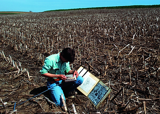
Grid sampling is a site specific mapping practice done by combining geo-referenced soil sampling and Geographic Information Systems (GIS). By utilizing a Global Positioning System (GPS) and an aerial photograph of a particular field, a sample grid is laid out based on a per acre grid. For a generalized representation of data, 2.5 acre grid cells are commonly used, though smaller ones are used for more precise results. By recording the GPS location of each sample, the same position may be used for future testing. When collecting soil samples, a device called a soil step probe is used to take a core of the soil at a depth of 8 inches. There are 5 cores taken in close proximity to the coordinate location to achieve a general representation of data. With the samples collected, they are sent to a University where they are tested for nutrient levels such as organic matter, pH, phosphorus, potassium, zinc, nitrate, or anything of interest to the farm operation.

 

Grid Data:

With the received test results, maps are created by interpolating between grid points using GIS for a visual representation of the data as shown in the maps below. The farm operation then uses the maps to determine areas of nutrient deficiencies and how much of and what fertilizers are needed for a desired soil fertility. The data itself is uploaded into a thumb drive where it is used for variable rate application in farm machinery. With map analysis complete, the thumb drive uploaded, and fertilizers ordered, a precise application of fertilizers makes it possible to raise the soil to an optimum fertility.

 

EC Mapping

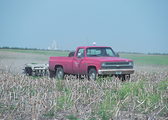
Another way to map soil variability with precision is through Electrical Conductivity (EC) mapping. EC is a technique used for on-the-go, GPS, soil mapping done with a machine rather than a labor intensive grid layout. The machine is simply pulled into the field by truck and the sensors lowered into the soil. This type of mapping uses electricity to determine how conductive the soil is. When the sensors are lowered into the soil, they emit electrodes which then surge through the soil and back to receiving electrodes to complete the circuit. An onboard computer analyzes how conductive the soil was through the measurement of voltage drop by subtracting the received energy from the initial output. The computer also loads the collected data into a map format for instant visualization. The variables collected include soil texture in reference to the actual soil type based on certain clays, sands and silt. This information is important for determining the water retention of the soil and the cation exchange related to pH levels. The pH regulates the nutrient exchange between the soil and plant. The more acidic the soil is the more it impedes the amount of nutrient transfer. The machine also creates a very precise map of actual soil textures by driving in dense linear passes across the field, covering the majority of the field area.

 

 

 

 

 

 

 

 

 

 

 

 

 

 

Mapping Techniques Drawbacks

Grid sampling provides many options in soil nutrient testing, but it can be an extremely expensive option to choose in order to receive information that was worth the time, money, and effort. The denser the grid is, the more precise the data will be in terms of the variability of the soil. While precision is important, it isn't cost effective to take that many samples. Though, if the grid is too coarse or limited, the data received can be a vague representation of the soil variability resulting in impractical information. The sampling process can take a lot of time as well. It has to be taken into consideration on whether it's worth the long hours of repetitive work in the heat of the day. Or if doing it your self isn't an option, it can be hired done, but it can still be an expensive service.

 

Electrical Conductivity mapping provides a very efficient technique, regarding the amount of time it takes, for mapping soil variability, but the equipment required for the process can be expensive. It must be taken into consideration the amount of land being mapped to determine the cost effectiveness of owning such a machine. From this type of technology it is also restrictive in providing information on a wide variety of variables that soil grid mapping does provide. This limits what a farming operation knows about their farm and what action to engage regarding fertilizer applications and initially leads to grid mapping in conjunction to EC mapping.

 

Remote Sensing:

By comparing these soil maps with remotely sensed data, a farm operation can determine why the nutrient levels remain the way they do. Imagery such as Light Detection and Ranging (LIDAR) or Digital Elevation Models (DEM), provides information on elevation and how water may be draining through the particular field of interest. Any correlation between low nutrient levels and poorly drained areas or excessively drained areas can be repaired to proper working order by the farm operation. An example of such maps is shown below.

 

 

 

 

 

 

 

 

 

 

 

 

 

 

 

 

 

 

                                       

 

Maps created by Justin Abel, Emporia State University student. The map shows a correlation of several soil nutrients and the LIDAR image including zinc, pH, and organic matter. The correlation is located in the center of the LIDAR image in the low elevation of the field.